How can I analyse my transcriptomics data in Mass Dynamics?

Upload your transcriptomics data

Transcriptomics data should be uploaded to Mass Dynamics using the supported transcriptomics MD input format, with raw gene expression counts provided as integer values rather than pre-normalized or log-transformed intensities.

After the data has been successfully uploaded, below are the suggested steps to help you get ready to analyse your data.

Exploratory data analysis and visualizations

For exploratory data analysis and visualization, we recommend first transforming raw counts to counts-per-million (CPM) and filtering poorly expressed genes using the Normalization & Imputation workflow (see section below: Create a filtered CPM dataset).

Log-CPM values are commonly used for dimensionality reduction and visualization in RNA-seq analysis (e.g. limma and edgeR workflow; Law et al. 2018), as they stabilize variance and support robust visualization. Visualisation modules in the app automatically apply log transformations where appropriate before plotting. This improves stability and interpretability for methods that are sensitive to highly skewed count distributions or zero inflation.

The filtered CPM dataset can then be used across visualization modules, including:

• Principal Component Analysis (PCA)
• Heatmaps
• Distribution plots
• Clustering visualizations

Some visualizations may fail or produce unstable results when raw count matrices with zeroes are used directly, particularly when downstream methods require or assume log-transformed input. Refer to this content page to understand the implications of zeroes and missing values in your data.

Create a filtered CPM dataset

Step1. Create a counts-per-million (CPM) dataset from raw gene expression counts

1. Go to the Dataset Creation page
2. Choose the Normalisation & Imputation dataset. From here it is possible to select the CPM normalisation option 
3. Click Create

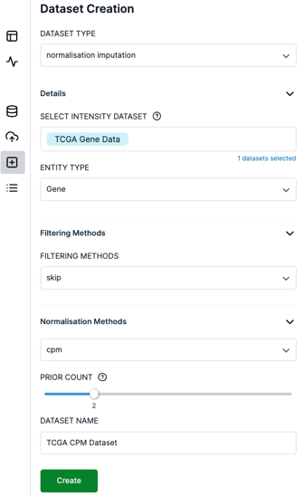
Setting prior counts to a value greater than zero (added to each expression value) is recommended to prevent taking the logarithm of zero in downstream visualisations and analyses.

Step 2. Filter lowly expressed genes using the newly created CPM dataset

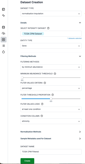
Filter genes based on a minimum CPM threshold and the minimum number of samples in which the gene must be detected. This follows recommended transcriptomics workflows such as limma-voom (Law et al. 2018).

Go again to the Normalisation & Imputation dataset creation and use the newly create CPM dataset to apply filtering. See examples of filters settings in the image below.

As a guide:

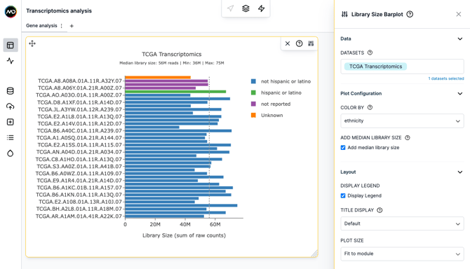
• Choose a CPM threshold based on the median library size of the experiment. For example, with a median library size of 20M reads, a CPM threshold of 0.5 is appropriate (equivalent to ~10 reads, i.e. 10/20). In Mass Dynamics you can explore the distribution of the library sizes in your dataset using the Library Size Barplot module.
• Choose the minimum number of samples based on the experimental design and number of replicates. A common approach is to require expression in at least 50% of replicates within the condition of interest.

Filtering setting example in the Normalisation & Imputation dataset creation page

Library Size Barplot module using an example dataset

On top of helping to choose a suitable CPM filtering threshold, inspecting library size distributions can also help determine the most appropriate differential expression workflow for the dataset. 

You can now safely use the filtered CPM dataset for visualizations like dimensionality reductions, heatmap, intensity distributions etc..!

Need to further normalise your data?

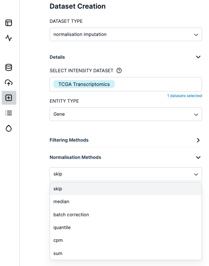
On top of the CPM transformation, Mass Dynamics has a variety of normalisation methods available in the Normalisation & Imputation dataset including two batch correction methods: the limma removeBatchEffect function (Ritchie et al., 2015) and combat (Johnson et al., 2007).

Choosing a differential expression engine

For transcriptomics data, the recommended workflow depends on the input data type:

• limma-trend (Law et al., 2014; Phipson et al., 2016) should be used when working with pre-normalized or log-scaled expression values such as filtered CPM data.

In Mass Dynamics, log transformation is applied automatically during the analysis step. Therefore, the required input for this engine is the filtered CPM dataset rather than pre-computed log-CPM values.

According to the limma R package documentation, the limma-trend workflow is recommended when library sizes are relatively consistent across replicates, with no more than approximately a 3-fold difference between the largest and smallest library sizes.

For datasets with highly variable library sizes, limma-voom is the standard alternative. While limma-voom is not yet implemented in Mass Dynamics, the following methods are recommended for this scenario.

• edgeR (Chen Y. et al 2025) and DESeq2 (Love MI et al. 2014) should be used when starting directly from raw integer gene expression counts. Both methods are highly stable with small sample sizes, i.e. very few replicates per condition and when library sizes are highly variable. 

edgeR and DESeq2 generally agree on strong differential expression signals. Differences are more commonly observed for low-count genes, where:

• • edgeR may behave more liberally
  • DESeq2 tends to be more conservative
  • and DESeq2 shrinkage methods can provide more stable fold-change estimates.

Once pairwise or ANOVA analyses are completed, the resulting outputs can be explored consistently across workflows using volcano plots, ANOVA volcano plots, and downstream visualization tools in the platform.

Filtering poorly expressed genes before differential expression

For transcriptomics workflows using limma-trend, we recommend using the filtered counts-per-million (CPM) dataset generated through the Normalization & Imputation workflow as described in the section above.

For workflows using edgeR or DESeq2, the original raw integer gene expression counts should be used directly as input. These pipelines include built-in low-count filtering based on edgeR’s filterByExpr method, which:

• is design-matrix aware,
• removes genes unlikely to achieve sufficient counts across the smallest condition group,
• and uses default thresholds of:
• min.count = 10
• min.total.count = 15

The same filtering is applied before both edgeR and DESeq2 analyses to ensure results are generated from the same gene set.

DESeq2 additionally performs independent filtering during statistical testing. Genes with very low average normalized counts may therefore receive NA adjusted p-values if they are unlikely to contribute statistically significant discoveries.

Genes removed during filtering remain visible in output tables but appear with NA statistics.